Foundations of computer programming in MATLAB — Introduction to functions

Introduction to functions

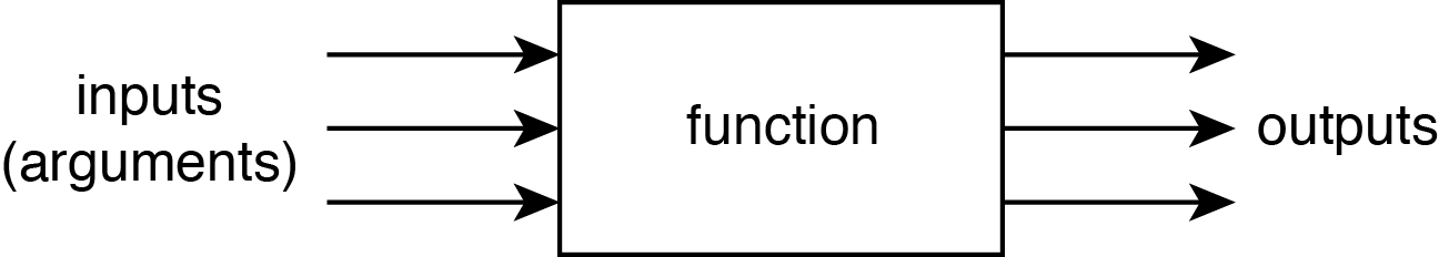
Functions allow us to use a process whenever it is convenient without having to rewrite the same process for new variables. Functions have inputs and outputs. The inputs are supplied to the function via the function’s arguments. When we call a function, it returns its outputs.

Even when we don’t know if a process we write will be reusable later, it can still be advantageous to write a function for it because this results in more clearly organized and understood programs. One reason this can be helpful is that functions provide local variables that have a limited scope and do not clutter up the primary script’s workspace, as we will see.

Types of functions

MATLAB gives us several basic function types, which we will take in turn. Most function types, such as main functions, local functions, nested functions, and private functions are written in a special type of file called a program file. These files are typically called from a primary program/script.

Program files

Program files all begin with a line such as the following.

function OUT = my_function(ARG1,ARG2)

The first word, function, must always appear at the beginning. The name of the output variable OUT is up to you, but it must appear immediately after function if you would like your function to return an output. The function name my_function is also up to you (caveat: it must be a valid MATLAB filename and variable name), but the program file name must be exactly the name of the function. The names of the arguments ARG1 and ARG2 are also up to you, and you may have as many as you like.

Main functions

The first line of the program file defines its main function. Besides the first line, the only other requirement of the program file is that it, if you’d like to have the output of the function returned, you must set the output variable. Finally, although it is not strictly necessary, it is good form to place end and the end of your main function.

Example

Let’s create our first function. Let it have two arguments, and let it return the smaller divided by the larger. If the are equal, let it return 1.

function out = small_divided_by_big(a,b)

if a < b
  out = a/b;
else
  out = b/a;
end

end

Let’s save this file in our current directory (Documents/MATLAB by default) with filename small_divided_by_big. In the Command Window, we should be able to try it out by entering something like the following.

small_divided_by_big(4,20)  % 0.2
small_divided_by_big(20,4)  % 0.2
small_divided_by_big(5,3)   % 0.6

Exercises

Write a program file with main function named raise_you_percent that takes two arguments: a “bet” value and the percentage $p$ you’d like to raise. It should return a single value: the original bet plus the raised amount.
Write a program file with main function named my_std that takes one argument: a numeric one-dimensional array. It should return the standard deviation of the array normalized by the number of elements minus one (the standard formula).
Write a program file with main function named three_rand_i_ten that takes zero arguments but returns three random integers between 1 and 10 as separate outputs.
Write a program file with main function named twelves that takes one argument: n. It should return an n by 1 array with all elements equal to 12.

Local functions

Some functions are really only useful to another function. Instead of starting an entirely new program file, a local function can be used. A program file can contain any number of local functions. The syntax is as follows.

function out = main_function(arg1,arg2)
...
dum = local_function(dum_arg);
...
end
function out_local = local_function(arg1_local)
...
end

Nested functions

Nested functions are very similar to local functions, but differ only in that they are placed inside the main function. The only difference is that a nested function has access to the variables inside the main function, whereas a local function does not, unless they are passed as arguments (or declared as global).

function out = main_function(arg1,arg2)
...
dum = local_function(dum_arg);
...
  function out_nested = nested_function(arg1_nested)
  ...
  end
end

Private functions

Private functions are just like regular program files, but they are limited in scope (which programs or functions can call it). They are saved in a subdirectory called private, and are only available to functions or programs located at the level above the subdirectory. More on these in a moment.

Anonymous functions

These handy little guys don’t require a separate program file! They accept inputs and return outputs, just like other functions, but they do have one limitation: they can contain only one executable statement. Therefore, they only work for simple functions like mathematical functions. Here’s an example.

my_times = @(arg1,arg2) arg1*arg2;

The variable my_times is now a function_handle data type. The arguments arg1 and arg2 are multiplied by each other and returned as the output. If you want to use the function, call it with the syntax my_times(3,4).

Exercises

Write an anonymous function called my_sin that is a sine wave and has the following arguments: amplitude A, angular frequency omega, and phase in radians phi, and a time array t. Try it out for a few values of each argument. Try it with the following parameters and plot it. <pre>% A: 2 ... omega: 2*pi ... phi: pi ... t: 0:0.01:2 t_array = 0:0.01:2; figure; plot(t_array,my_sin(2,2*pi,pi,t_array));</pre>
Write an anoymous function my_square, just like my_sin, except that it is a square wave instead of a sine wave. Hint: use the mod function and a conditional statement. Plot with the my_sin example as follows. <pre>% A: 2 ... omega: 2*pi ... phi: pi ... t: 0:0.01:2 t_array = 0:0.01:2; figure; plot(t_array,my_sin(2,2*pi,pi,t_array),'b'); hold on; plot(t_array,my_square(2,2*pi,pi,t_array),'r');</pre>

Function precedence order

The MATLAB path

You may have encountered what is called the path for your operating system, before. This is simply a collection of directory names where your operating system looks for programs you tell it to execute (typically from the command line). We can add directories to the path whenever we like, but we must be cautious not to give the operating system too many places to look, or it can slow down the execution of programs. Moreover, we might have multiple programs in our path with the same name. If this occurs, the operating system falls back on function precedence order, which will be addressed in a moment.

MATLAB has its own path where it looks for MATLAB programs and functions. This should help explain that previously mysterious dialog box you’ve seen when first executing your program.

The current directory

In addition to the path, MATLAB will look in your Current Directory for programs. This can be any directory you like. Navigate to it via the Current Folder view. The Current Directory does not automatically get added to the path, so you can run programs from it without cluttering up your path. We usually don’t add our Current Directory to our path.

Precedence of functions

Finally, we can understand what is meant by “function precedence.” When a variable is evaluated by the interpreter, it uses the following precedence order:

variables in the current workspace;
imported package functions (using import);
nested functions;
local functions;
private functions in the subdirectory private of the Current Directory;
object functions;
class constructors in @ directories;
loaded Simulink models;
functions in the Current Directory; and
functions elsewhere in the path, in order of appearance.